Getting started with the Sandbox

Introduction

The QCentroid platform includes a cloud hosted development environment base on Jupyter Notebook.

This environment is ususally refered as the IDE or sandbox.

Start using the IDE:

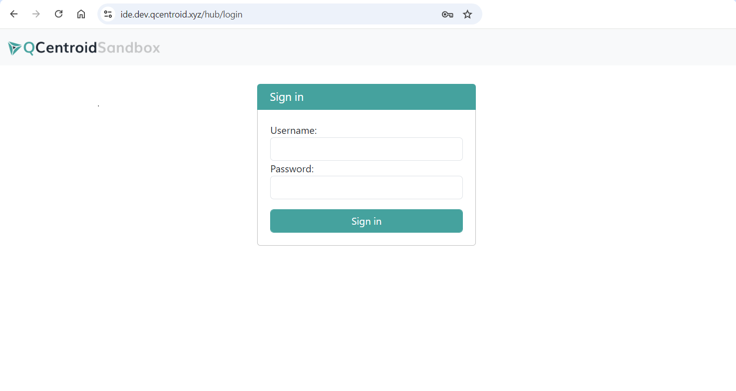
1. Access the Development environment through this URL: https://ide.dev.qcentroid.xyz/

   • Use your email address and password

   

2. Your server starts automatically.

   • After the login, a Jupyter server will launch automatically. You’ll have a 16 cores and 32GB memory environment to develop and run your solution.

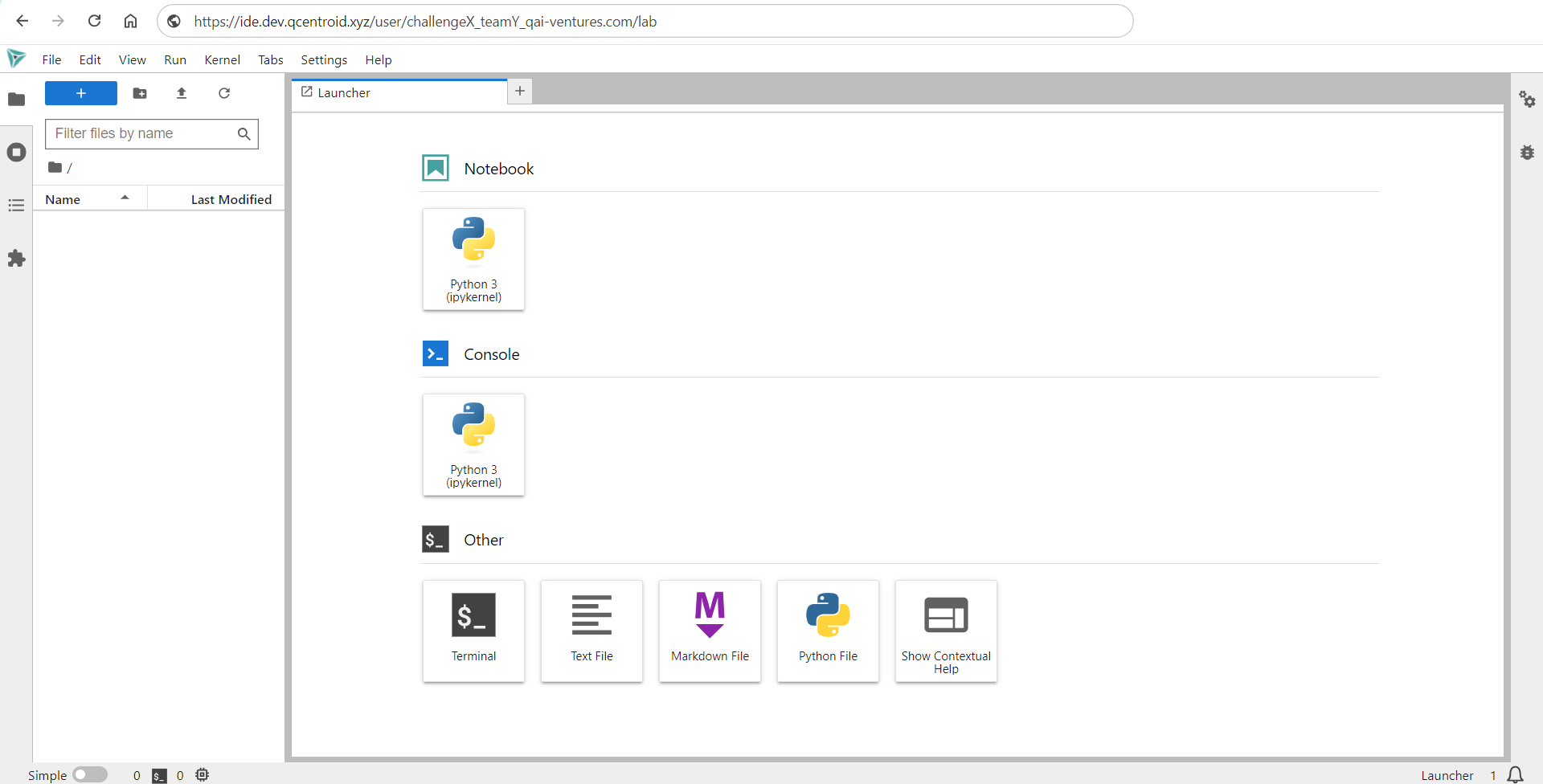
3. You will be redirected to your Jupyter Notebook development environemnt after the login.

   

4. You will see that the IDE is connected to your GitHub repository and your source-code template is already there.

Using the Sandbox

Implement your solvers using the Solver Template

Once the use case has been choosen and you have registered a solver in the platform, you can start implementing the actual source code of your solver.

Let’s see how we can implement the solver in a way that it can run on IDE and on the QCentroid platform.

Understand the solver template

The solver template contains two main files:

• Launcher.ipnpy Jupyter notebook to test and run your solver in the IDE
• main.py Main solver file that contains the algorithm

The following subsections describe the files that you will find in the repository.

Launcher.ipnpy

This is the Jupyter Notebook that you can use in the IDE environment to run and test your algorithm.

It contains additional instructions and all the necessary steps.

main.py

This file will contain the solver itself.

It also has a run() function with a specific signature that receives these paramters: input_data, solver_params and extra_arguments.

This is your solver entry point. Do not modify it.

main.py

import logging
logger = logging.getLogger(__name__)

from qiskit import QuantumCircuit, Aer, execute, IBMQ

def run(input_data, solver_params, extra_arguments):

    logger.info("Starting Solver...")

    # Here goes your solver's code

    logger.info("Ending Solver...")
    output = {}

    output["output_param"] = "This is an output parameter"

    # And this is the output it returns
    return output

The input_data parameter contains the input data of this job execution, whether it is a local JSON file provided from the Launcher notebook, or provided when executing a job in the Quantum Platform.

Modify the solver source code

You will want to start modifying the template in the main.py file.

This file contains the run() function which is the entry point.

From this point you can start modifying the sample code and adding your own algorithm.

How to handle exceptions

Important

Do not catch exeptions globally in your solver. Let blocking exceptions to raise and to be handled by the platform for you, so the execution is stopped and the exception message is shown in the dashboard.

You can add limited scope exception handling in your solver code, but make sure to raise blocking errors as exceptions so the platform can capture them and stop the execution.

You can check this exceptions in the dashboard in the job details page after the execution.

How to add logs to your solver

You can add logs in your solver and see them in the platform web dashboard after every execution.

Tip

Add as many logs as you want, specially during the development, testing and experimentation phases to gather as much information as possible of your solver’s performance.

To do this, do the following in any of your solver files:

First, import Python’s native library for logging and initialize it:

import logging
logger = logging.getLogger(__name__)

Then, add as many log records as you want throughout your code:

logger.info("Starting solver execution...")

This is an example of a main.py file that includes log records:

main.py

import logging
logger = logging.getLogger(__name__)

def run(input_data, solver_params, extra_arguments):

    logger.info("Starting solver execution...")

    # This is your solver's code:

    input_param_1 = int(input_data['param_1'])

    logger.info(f"Input param_1: { input_param_1 }")

    output = {"output_param": "This is an output parameter"}

    # And this is the output it returns
    logger.info("End of solver execution.")

    return output

All these log records are stored and displayed in the web dashboard in the job details page, in the Execution logs tab.

How to measure execution time

You can use this logging feature to measure your solver’s effective execution time by using the time library

Tip

You can measure the execution time of your solver or any subprocess within your solver.

Import Python’s native time library:

import time

Record the start and end time, substract them and send it to the execution log:

start_time = time.time()  # Start timing

# The process you want to measure

end_time = time.time()  # End timing

elapsed_time = end_time - start_time

logger.info(f"Elapsed time (in seconds): { elapsed_time }")

Run the solver in the IDE

To run your solver in the IDE during the development process and before uploading it to the platform, just use the provided Jupyter notebook (the Launcher.ipnpy).

3. Push the code to GitHub

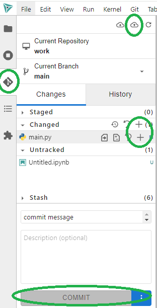
When you have a working version of your solver, track, stage, commit and push the code to the GitHub repository from the left sidebar of the IDE.

To do this:

1. Click on the Git tab on the left toolbar
2. For new added new files, track and stage them by clicking on the plus (+) button next to your untracked files
3. For modified files, use the plus (+) buttons next to the changed files to stage them
4. Write a commit message and click the COMMIT button
5. And latsly, click the Push button at the top-right corner of the panel to send the changes to the server.

At this point, your source code is stored in GitHub and it can be transfered (Pull and build) to the platform.

4. Pull the new solver code into the platform

Now that you have your solver source code tracked in a repository, you can Pull and build it into the plaform to be able to run jobs with it.

Go to the Repository details page via the left-side menu, Solvers > Repositories, then click on your repository, and click the Pull & build button next to your solver.

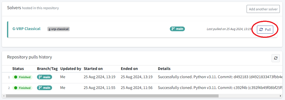
Below, you can check the builds history. Just wait until this process is shown as Finished and make sure the commit used is the one that you just pushed to GitHub.

Now, your solver is ready to run jobs in the platform.

5. Run your solver in the platform

The last step will be to run the solver that you just created in the platform.

With QCentroid’s no-code executions feature, you can launch jobs directly from the platform dashboard.

To launch a job:

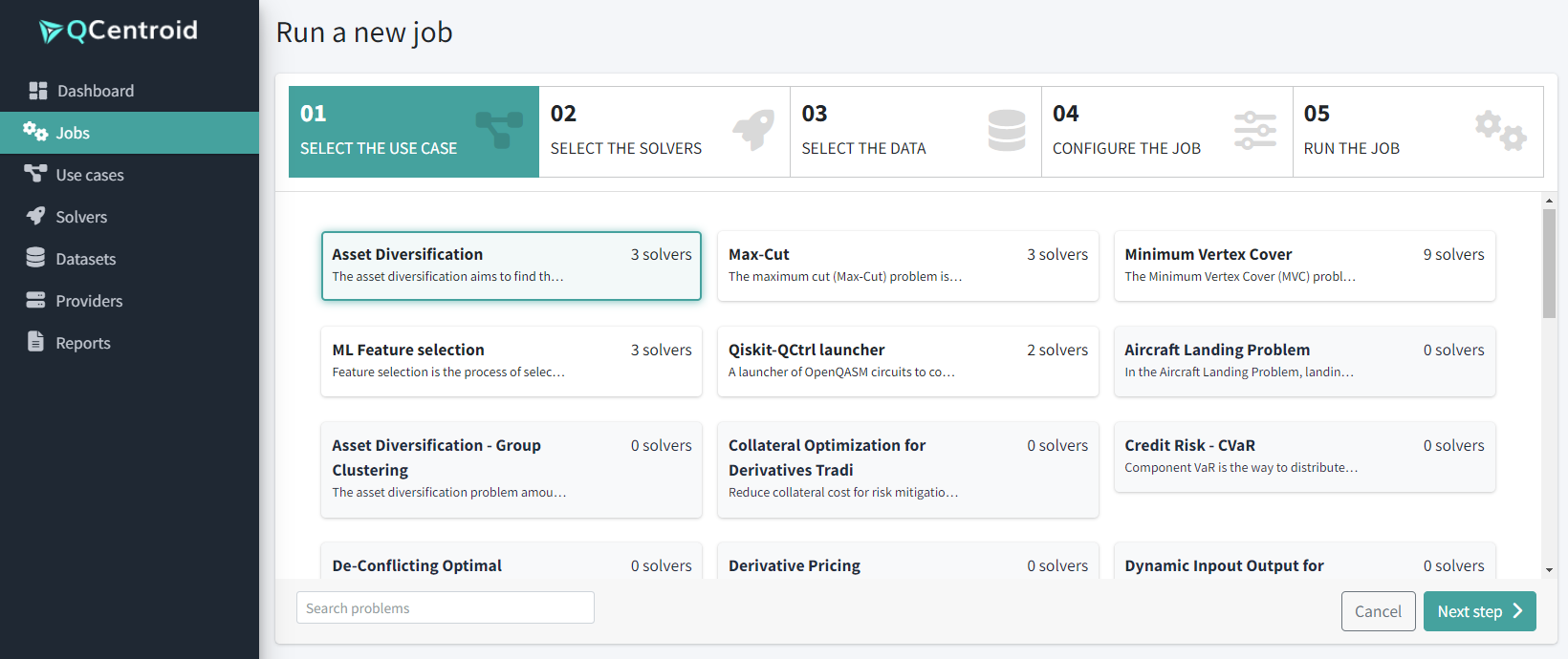
1. Navigate to the Jobs section via the left-side menu.

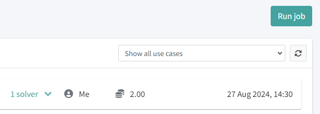
2. Click the Run job button, and proceed with the wizzard.

   

3. Select the Use case:

   

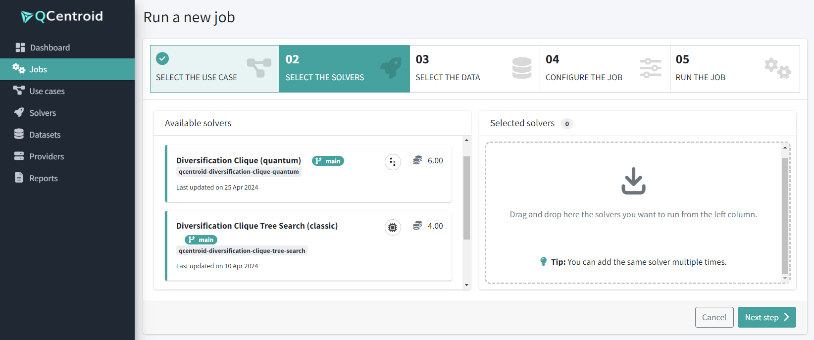
4. Select your solver (drag and drop it to the right side):

   

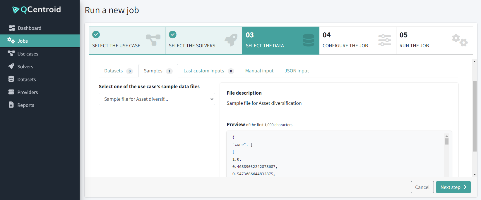
5. Select the input data for this execution from any of the sample datasets.

   

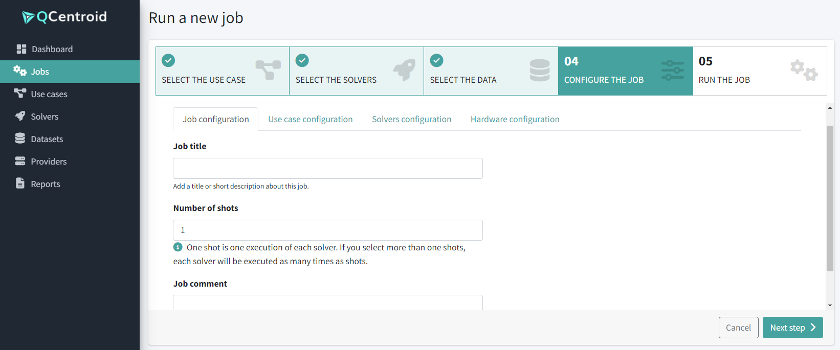
6. Write the job’s description and comment:

   

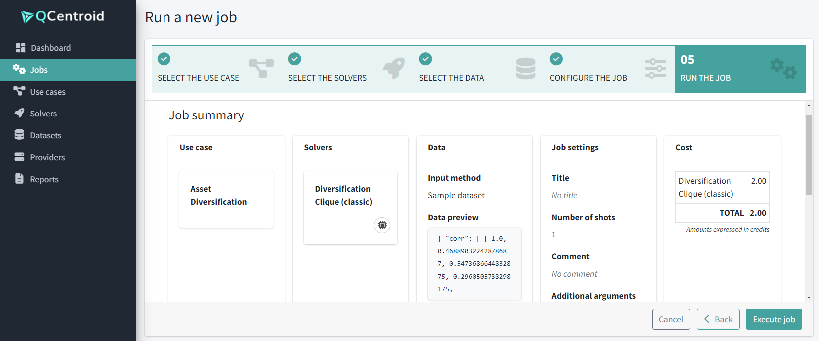
7. Review the job summary:

   

8. And click the Execute job button.

You will receive a notification on the top-right corner confirming that a new job has been launched.

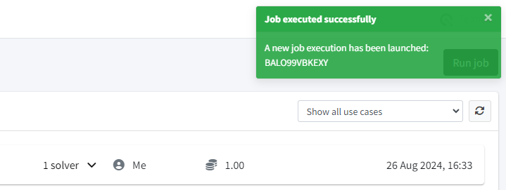
Just wait untill the job is in status Finished and click on it to see the job results.

Click the Raw results tab to see either the solver output for successfull jobs or the error trace if it failed.